Frame-Aligned Records
Exact safeguards for locality-record comparisons
James McGaughran
MathGov / RippleLogic Research Program
26 September 2026 | Review manuscript v0.5
Abstract
Which subsystem descriptions make quantum dynamics simple, and which support informative records? We develop three safeguards for comparing them: access-aware equivalence, valid inferential targets, and uncertainty-aware record certification. A centred projection score is bounded and energy-origin invariant. Covariant preparations obey spectral-block restrictions, while conditional typicality constrains state-adaptive selection within a predetermined, quantitatively bounded family. Equal higher-weight operator spans need not define equal access, restricted permutation references can be miscalibrated, and unequal certificate tightness must not become an apparent physical advantage. A source-off pilot illustrates why the estimand matters. Its predeclared six-qubit readability-change mean is negative, -0.015225. A subsequent paired factorial extension instead compares two Hamiltonian orientations at fixed injection and finds positive intervention contrasts, approximately 0.0105 and 0.0126 at six qubits. Reproduction and a finite-family variance-sensitive analysis support those contrasts under the specified sampling law. The two signs are compatible because their counterfactuals differ. Rotating the Hamiltonian is not an intervention on locality alone, and finite propagation bounds do not establish the sign of this readability statistic. The paper supplies reusable comparison safeguards, not a new decoherence mechanism, an identified spacetime metric or a consciousness result.
Keywords: quantum mereology; quantum records; conditional typicality; locality; statistical inference; reproducibility.
1. Introduction
1.1 The question
Decoherence and quantum Darwinism explain how certain observables of a system become stably and redundantly recorded in an environment, given a decomposition of the global Hilbert space into system and environment [Zurek 2003; Ollivier, Poulin and Zurek 2004; Zurek 2009]. The decomposition itself is usually supplied. Work on quantum mereology asks where it comes from: which tensor-product structures (TPS) are singled out by a Hamiltonian, a state, or an operational criterion [Zanardi 2001; Zanardi, Lidar and Lloyd 2004; Cotler, Penington and Ranard 2019; Carroll and Singh 2021; Zanardi, Dallas, Andreadakis and Lloyd 2024]. Two families of criteria have been developed largely in parallel. Locality criteria select structures in which the Hamiltonian is a sum of few-body or graph-local terms. Classicality criteria select structures that host robust pointer states or redundant records [Riedel 2017; Adil et al. 2026].
A natural question joins them: across an ensemble of models, do the candidate structures that are nearly optimal for dynamical locality coincide with those that are nearly optimal for persistent, informative records more often than a declared chance baseline predicts? We call this the locality-record compatibility question. It is implicit in programmes that seek to recover classical, spatially organised descriptions from minimal quantum ingredients, with conditional model-class formulations stated in Section 7. Recent results pull in different directions. Riedel showed that, given the TPS associated with spatial locality, the requirement of redundant local records strongly constrains branch decompositions [Riedel 2017]. Adil et al. found that a fixed Hamiltonian can admit many factorizations with robust pointer states, and that decohering subsystems need not align with the usual notion of locality [Adil et al. 2026]. Whether a Hamiltonian alone determines a TPS is itself disputed [Stoica 2022; Soulas, Franzmann and Di Biagio 2025; Stoica 2026].
1.2 Why the question is easy to trivialise
A test of compatibility must score many candidate structures under one physical history and compare the two sets of near-optimal candidates. Three choices can decide the outcome before any physics is done.
The score may be ill-posed. An uncentered numerator divided by the centered Hamiltonian norm is unbounded when its orthogonal projection omits the identity; candidates that differ only by a local unitary or a relabelling may be counted as distinct and inflate overlap.
The preparation may be uninformative. A deterministic, fully covariant Hamiltonian-only preparation is stationary under that same autonomous Hamiltonian. This does not exclude pre-existing records or conditional dynamics hidden by a stationary average. Under conditional Haar assumptions, qualification becomes unlikely in a specified small-fragment regime, but is not impossible (Proposition 3).
The null may be miscalibrated. A uniform pairing of candidate labels mistakes duplicated candidates for independent opportunities, and a recording-friendly design with the preparation, coupling and dynamics aligned can build much of the desired coincidence into its inputs. Alignment alone does not guarantee records for every Hamiltonian or time window.
1.3 Contributions
Three failure modes organize the contribution.
- Mistaking a convenient description for an equivalent physical access structure. The centred score and full operational stabilizer make comparisons well posed. The controlled-NOT counterexample shows why equal higher-weight spans alone do not suffice (Sections 2 and 3).
- Mistaking an analysis convention for evidence. Explicit reference assumptions, the exact derangement counterexample, and the distinction between a change from frozen evolution and a paired Hamiltonian-orientation intervention prevent different questions from borrowing each other’s verdicts (Sections 5 and 6).
- Mistaking a numerical limitation for absent records. Lower and upper count bounds propagate unresolved certification into inference. Conditional preparation and finite-cover results delimit when a chosen search family can find records (Section 7.3.1; Appendices C to F).
Elementary lemmas and standard concentration tools support these safeguards. The methodological integration and the finite design examples are the contribution claimed here; historical priority for a new physical mechanism or for the underlying mathematics is not claimed. Unrestricted structure recovery and the persistent-count population conjectures remain unexecuted.
2. Setting and definitions
2.1 System, source and reference structure
Let \(\mathcal H_S=(\mathbb C^2)^{\otimes n}\) with \(d=2^n\), and let \(\mathcal B(\mathcal H_S)\) carry the Hilbert-Schmidt inner product \(\langle A,B\rangle =\mathrm{Tr}(A^\dagger B)\) and norm \(\|A\|_2\). A classical binary source \(X\in\{0,1\}\) with prior \((p_0,p_1)\) is held in a separate register that is never rotated by a candidate. Equivalently, a source qubit prepared in a \(Z\) eigenstate couples through \(Z_{\mathrm{src}}\otimes K\).
A reference structure \(\mathcal R=(S,\{\mathcal A_F\}_F,\mathcal Q)\) comprises a declared local operator span \(S\), eligible fragment algebras \(\mathcal A_F=\mathcal B(\mathcal H_F)\otimes I_{\bar F}\), and an operational contract \(\mathcal Q\). The contract records fragment-size limits, disjointness, source exclusion, allowed measurements, access costs, and any graph or site labels. The symbol \(\mathcal B(\mathcal H_F)\) denotes the full matrix algebra; the standalone contract \(\mathcal Q\) is metadata, not another algebra. All projections onto operator spans are Hilbert-Schmidt orthogonal.
A candidate represented by a unitary \(V_D\) rotates both the local span and the fragment algebras, with the contract transported consistently. The full stabilizer is \[\mathrm{Stab}(\mathcal R)=\{W\in U(d):\operatorname{Ad}_W(\mathcal R)=\mathcal R\}.\] Here equality means preservation of the local span, permutation of the eligible fragment algebras, and preservation of every applicable element of the operational contract. Thus \(V\) and \(VW\), with \(W\in\mathrm{Stab}(\mathcal R)\), define equivalent candidates. Equality of a locality span alone does not suffice. Source registers remain external and are not accessible fragments.
For \(n\) equal-dimensional sites (site dimension \(q_{\mathrm{site}}=2\) in the qubit models) with every singleton algebra, unrestricted singleton measurements, symmetric costs, unlabelled sites and an unrestricted weight-\(k\) span, the stabilizer is exactly the set \[\{\Pi_\pi(U_1\otimes\cdots\otimes U_n):\pi\in S_n,\ U_j\in U(q_{\mathrm{site}})\}.\] This set notation avoids treating the product of local unitary groups as an injective subgroup: compensating local phases have a kernel. Graph or operational constraints restrict the allowed elements further. In the unlabelled case these are the usual TPS equivalences; a labelled or cost-restricted access structure has a finer equivalence relation [Andreadakis and Zanardi 2025, Eq. 14 and Appendix A.4].
2.2 Convention for evaluating candidates
For any operator \(A\) and unitary \(V\), \[\Pi_{VSV^\dagger}(A)=V\,\Pi_S(V^\dagger AV)\,V^\dagger,\qquad(1)\] because \(A\mapsto VAV^\dagger\) is a Hilbert-Schmidt unitary that maps \(S\) onto \(VSV^\dagger\) and \(S^\perp\) onto \((VSV^\dagger)^\perp\). Consequently, scoring the physical operator \(A\) against the rotated structure \(\mathcal R_D\) is the same as scoring \(A_D:=V_D^\dagger AV_D\) against the fixed reference structure. We use the second form throughout: \[H_D:=V_D^\dagger HV_D,\qquad \rho_D(t):=V_D^\dagger\rho(t)V_D.\] Every candidate is evaluated on the same physical history. Jointly conjugating the Hamiltonian, the state, the observables and the reference structure by one unitary leaves every score unchanged; it is a recovery check, not a candidate. Changing only the state, or only the Hamiltonian, defines a different physical experiment.
2.3 Dynamics
The record-generating dynamics is a source-conditioned family of autonomous Hamiltonians \[H_x=H_S+K_x,\qquad x\in\{0,1\},\] where \(H_S\) is the internal Hamiltonian and \(K_x\) the source coupling (in the historical continuously driven calibration, \(K_x=(-1)^xK_{\mathrm C}\)). A preparation law \(\mathsf P\) is a probability law over \((H_S,K,\rho_x(0))\), and the source-conditioned states are \(\rho_x(t)=e^{-iH_xt}\rho_x(0)e^{iH_xt}\). When the initial state does not depend on \(x\) we write \(\rho(0)\). The symbol \(K_{\mathrm C}\) denotes a coupling operator; C in \(D_C\), \(U_C\) or \(H_C\) labels the alternate frame.
2.4 Locality score
For Hermitian \(H\) let \(H_0=H-\mathrm{Tr}(H)I/d\). Let \(S_0\) be a declared traceless Hermitian operator space and let \(S=\operatorname{span}\{I\}\oplus S_0\). The canonical score is \[L_S(H)=\frac{\|H_0-\Pi_{S_0}(H_0)\|_2^2}{\|H_0\|_2^2},\qquad H_0\ne0.\qquad(2)\] All projectors here are Hilbert-Schmidt orthogonal. The legacy uncentered expression is denoted \(L^{\mathrm{raw}}_S(H)=\|H-\Pi_S(H)\|_2^2/\|H_0\|_2^2\). For identity-inclusive \(S\) these are identical. Lemma 1 states the precise domain of that equivalence; the two forms are not independent measurements. A scalar Hamiltonian (\(H_0=0\)) receives UNINFORMATIVE_SCALAR. Numerical near-scalar exclusions use a declared absolute tolerance in stated input units, not one inflated by an arbitrary identity energy shift. A scalar source branch blocks the stated total normalized score unless an alternative aggregation was specified before analysis. Larger \(L\) means more weight outside the local span, so a locality threshold is a ceiling. For a candidate, \(L(D;H):=L_S(H_D)\). Two versions enter the analysis and must be declared in advance:
- internal locality, \(L^{\mathrm{int}}(D)=L(D;H_S)\);
- total locality, \(L^{\mathrm{tot}}(D)=\sum_xp_x\,L(D;H_x)\).
Supplement Section S2.6 shows how the choice changes the descriptive verdict in the historical continuously driven calibration.
2.5 Records
For fragment \(F\), candidate \(D\) and time \(t\), the conditional fragment states are \(\rho^{D}_{F,x}(t)=\mathrm{Tr}_{\bar F}\,\rho_{x,D}(t)\). The optimal probability of error in guessing \(x\) from \(F\) is the Helstrom error [Helstrom 1969] \[p_{\mathrm{err}}(F,D,t)=\tfrac12\bigl(1-\|p_0\rho^D_{F,0}(t)-p_1\rho^D_{F,1}(t)\|_1\bigr),\qquad(3)\] which for equal priors is \(\tfrac12-\tfrac14\|\rho^D_{F,0}-\rho^D_{F,1}\|_1\). With unrestricted measurements on \(F\), the bound is attained by a projective measurement of the weighted difference. Restricted or costly decoders require their own attainable error; fragment size alone does not certify that physical access is available. The Holevo quantity \(\chi(X{:}F)\) is an upper bound on accessible information, not an achieved value [Wilde 2019]; we therefore qualify records by (3). A fragment qualifies at tolerance \(\varepsilon\) over a window \(T_w\) if \(p_{\mathrm{err}}(F,D,t)\le\varepsilon\) for all \(t\in T_w\). The record score \(R(D)\) is the largest number of pairwise disjoint qualifying fragments within a declared fragment-size limit. Disjoint fragments may still be correlated; stronger objectivity notions such as spectrum broadcast structure require additional conditions [Horodecki, Korbicz and Horodecki 2015; Le and Olaya-Castro 2019, 2021]. A prior with \(\min_xp_x\) near zero makes a small error uninformative, so the source prior is part of the declared design. For a formation claim, declare an initial-error floor on the same fragments: \(p_{\mathrm{err}}(F,D,0)\ge\min(p_0,p_1)-\epsilon_0\), and then require persistent final error at most \(\varepsilon<\min(p_0,p_1)-\epsilon_0\). Let \(R_{\mathrm{new}}(D)\) count only fragments satisfying both conditions. A change in total count alone is insufficient: old records can disappear while different fragments acquire new ones. The presence score \(R\) and formation score \(R_{\mathrm{new}}\) remain distinct. Pointwise optimal decoding assumes knowledge of readout time and permits its decoder to vary; Appendix D states the stronger fixed-decoder alternative and the continuum certificate.
2.6 Near-optimal sets and the association event
With parameters frozen before scoring, \[\mathcal N_L=\{[D]:L(D)\le\tau_L,\ L(D)\le\min_{D'}L(D')+\epsilon_L\}.\]
\[\mathcal N_R=\{[D]:R(D)\ge\tau_R,\ R(D)\ge\max_{D'}R(D')-\epsilon_R\}.\] The association event for one sampled model and history is \(A=\mathbb 1[\mathcal N_L\cap\mathcal N_R\neq\emptyset]\). Empty sets stay empty; a model with no qualifying records has \(A=0\) and remains in every denominator.
2.7 Span similarity, access equivalence and numerical clusters
A candidate includes both a locality span and an access structure. Their stabilizers can differ. For equal-rank operator-space projectors define \[\delta_S(D,E)=1-\frac{\operatorname{Tr}(P_D P_E)}{r}=\frac{\|P_D-P_E\|_{\mathrm{HS}}^2}{2r}.\] This is a squared projector discrepancy. Its square root is a distance on the rank-\(r\) projector space. Neither expression alone identifies the full locality-and-access structure. The construction is related to operator-subspace geometry, but is not automatically the same object or theorem as the tensor-product-structure measures of Andreadakis and Zanardi (2025).
Exact counterexample 1: proximity is not equivalence. Rotate \(\operatorname{span}\{I,Z\}\) about the \(Y\) axis through Bloch angles \(0,0.2,0.4\). Consecutive discrepancies equal \(0.0197347515\), while the endpoint discrepancy is \(0.0758233227\). Thus \(\delta<0.03\) is not transitive. Also the squared discrepancy violates the triangle inequality in this example. Exact equivalence is assessed by a declared stabilizer. Approximate groups are called clusters and need a deterministic clustering algorithm, a tie rule and threshold sensitivity; they are never silently substituted for mathematical quotient classes.
Exact counterexample 2: equal spans need not give equal records. On two qubits let the allowed span be the complete operator space, so every conjugation leaves it unchanged. Compare the identity and controlled-NOT representatives, and source-conditioned vectors \(\left| 00\right\rangle ,\left| 11\right\rangle\). The identity access structure has two perfect single-qubit records. In controlled-NOT coordinates the vectors are \(\left| 00\right\rangle ,\left| 10\right\rangle\), giving one. The span discrepancy is zero in both cases. This is an access counterexample, not creation or destruction of information by a passive representation change.
Access equivalence from an existing theorem. Define \[\mathcal W=\operatorname{span}\{I\}+\sum_j\mathcal B_0(\mathcal H_j),\qquad r_1=\sum_j(q_{\mathrm{site},j}^2-1),\] where site algebras are embedded in the full system and \(\mathcal B_0\) denotes their traceless parts. If \(P_V\) projects onto \(V\mathcal W V^\dagger\), the Andreadakis-Zanardi squared TPS discrepancy is \[\Phi(V,W)=\frac{\|P_V-P_W\|_{\mathrm{HS}}^2}{2r_1}.\] Their Eq. 14 proves that \(\Phi=0\) precisely for a relative unitary consisting of local unitaries and permutations of equal-dimensional sites. The square root of \(\Phi\) is the associated projector distance; \(\Phi\) itself is a squared distance and need not satisfy the triangle inequality. The distinction is terminological, not a criticism of their convention. For two-qubit identity versus controlled-NOT, \(\delta_1=4/7\) when the identity is included in the rank, while \(\Phi=2/3\). SWAP has \(\Phi=0\) for unlabelled sites. These normalization differences must not be mixed.
This closes the ordinary unlabelled singleton TPS test. It does not replace the full contract when sites have different access costs, graph roles or restricted decoder sets. A site-permuting unitary can have zero \(\Phi\) while violating those labels. In that case retain the tuple of individual fragment-algebra projectors, minimizing only over permitted permutations, together with the locality and access metadata. Small nonzero \(\Phi\) is not an exact equivalence relation.
3. Structural lemmas for the locality score
Lemma 1 (boundedness and equivalent conventions). The centered score (2) lies in \([0,1]\). For an arbitrary orthogonal operator-space projection, \(0\le L^{\mathrm{raw}}_S(H)\le1\) for every non-scalar Hermitian \(H\) if and only if \(I\in S\). In the latter case the raw and centered scores agree and \[L_S(H)=1-\frac{\|\Pi_S(H_0)\|_2^2}{\|H_0\|_2^2}.\qquad(4)\]
Proof. Suppose \(I\in S\) and write \(H=cI+H_0\). Then \(\Pi_S(H)=cI+\Pi_S(H_0)\), so \(H-\Pi_S(H)=H_0-\Pi_S(H_0)\). Since \(\Pi_S\) is an orthogonal projector, \(\|H_0-\Pi_SH_0\|_2^2=\|H_0\|_2^2-\|\Pi_SH_0\|_2^2\in[0,\|H_0\|_2^2]\), which gives (4) and the bound. Conversely, suppose \(I\notin S\), so \(r:=(1-\Pi_S)I\ne0\). Fix any non-zero traceless Hermitian \(G\) and let \(H_\varepsilon=I+\varepsilon G\). The numerator of the raw expression is \(\|r+\varepsilon(1-\Pi_S)G\|_2^2\to\|r\|_2^2>0\) as \(\varepsilon\to0\), while the denominator is \(\varepsilon^2\|G\|_2^2\to0\). Hence \(L^{\mathrm{raw}}_S(H_\varepsilon)\) is unbounded. \(\square\)
Example. For \(n=3\), \(S\) the span of weight-one Pauli strings (identity excluded) and \(H=I+0.05\,X\otimes X\otimes I\), the numerator is \(\|I\|_2^2+\|0.05\,XXI\|_2^2=8.02\) and the denominator is \(0.02\), so \(L^{\mathrm{raw}}_S(H)=401\). Adding the identity to \(S\) gives \(L_S(H)=1\), as this \(H_0\) lies entirely outside the weight-one span (Supplement run S02).
Corollary 1.1 (affine invariance). If \(I\in S\) then \(L_S(aH+bI)=L_S(H)\) for all real \(a\ne0\) and \(b\). This is invariance of the score. Rescaling the Hamiltonian while holding clock time fixed generally changes record dynamics. Dynamical equivalence requires the corresponding time rescaling; an energy-origin shift of one autonomous branch only adds its global phase.
Lemma 2 (candidate-invariant denominator). For every unitary \(V\), \(\|(V^\dagger HV)_0\|_2=\|H_0\|_2\). Hence, with \(I\in S\), \(L(D;H)=1-\|\Pi_S(V_D^\dagger H_0V_D)\|_2^2/\|H_0\|_2^2\), and ranking candidates by \(L\) is ranking them by the local weight they capture.
Proof. \(\mathrm{Tr}(V^\dagger HV)=\mathrm{Tr}\,H\), so \((V^\dagger HV)_0=V^\dagger H_0V\), and the Hilbert-Schmidt norm is unitarily invariant. \(\square\)
Lemma 3 (class functions). If \(W\in\mathrm{Stab}(\mathcal R)\) then \(L(VW;H)=L(V;H)\) for every \(H\), and \(R\) computed with the fragment family of \(\mathcal R\) satisfies \(R(VW)=R(V)\).
Proof. Conjugation by \(W\) is a Hilbert-Schmidt unitary that maps \(S\) onto itself and hence \(S^\perp\) onto itself, so it commutes with \(\Pi_S\). Therefore \(\|\Pi_S(W^\dagger AW)\|_2=\|W^\dagger\Pi_S(A)W\|_2=\|\Pi_S(A)\|_2\) with \(A=V^\dagger H_0V\), and Lemma 2 fixes the denominator. For records, the full stabilizer must additionally preserve fragment sizes, disjointness, source exclusions and declared decoder/access budgets. Under these conditions \(W\) maps each fragment algebra onto an eligible fragment algebra of the same size, so eligible fragments correspond bijectively and paired reduced states are related by a common local unitary. The permitted decoder is transported with that correspondence. Attainable Helstrom errors, qualification decisions and the maximal disjoint count are therefore preserved; the reduced matrices need not be literally identical. \(\square\)
Numerically, for random \(8\times8\) Hamiltonians the change in \(L\) under a product of single-qubit unitaries, a cyclic qubit permutation, and their product is at most \(6\times10^{-17}\), while a generic unitary changes \(L\) by \(0.144\) in the sampled instance (Supplement run S02).
Consequence for counting. Candidate families must be reduced to classes before \(\mathcal N_L\), \(\mathcal N_R\) or any chance baseline is formed. Otherwise a family containing \(m\) stabilizer-equivalent copies of one structure offers \(m\) spurious opportunities for overlap. Section 5.3 quantifies the effect on the null.
3.1 Rank and fitting budget
For an isotropic unit direction in the real traceless-Hermitian space of dimension \(m=d^2-1\), an independently fixed rank-\(r\) orthogonal projector gives \[\mathbb E[L]=1-r/m,\qquad \operatorname{Var}(L)=\frac{2r(m-r)}{m^2(m+2)}.\] The mean follows from the isotropic second moment; the variance follows from the beta distribution of a projected spherical direction. A Haar-conjugated fixed traceless Hamiltonian has the same mean by adjoint irreducibility, but need not have that spherical variance. Fitting a projector to the same Hamiltonian changes the selection problem. Rank, admissible graphs and search effort must therefore be controlled or reported. A larger operator span is not evidence of a more meaningful recovered geometry merely because it leaves a smaller residual.
4. Preparation constraints
4.1 Proposition 1: covariance and stationarity
Let \(F\) be a deterministic rule assigning a density operator to a Hamiltonian on \(\mathcal H_S\), and write \(U_t=e^{-iHt}\).
Proposition 1.
\(F\) is covariant under the flow of \(H\), that is \(F(U_tHU_t^\dagger)=U_tF(H)U_t^\dagger\) for all \(t\), if and only if \([F(H),H]=0\), which is the statement that \(F(H)\) is stationary under \(U_t\).
If \(F\) is covariant under all unitaries, \(F(UHU^\dagger)=UF(H)U^\dagger\), then \(F(H)=\sum_\lambda f_\lambda P_\lambda\), where \(H=\sum_\lambda\lambda P_\lambda\) is the spectral decomposition. In particular \(F(H)\) is stationary and is uniform on each degenerate eigenspace.
A rule that selects a pure state inside a degenerate eigenspace can be stationary without being covariant under all unitaries.
Proof. (a) Since \(U_tHU_t^\dagger=H\), flow covariance reads \(F(H)=U_tF(H)U_t^\dagger\) for all \(t\). Differentiating at \(t=0\) gives \([H,F(H)]=0\). Conversely, if \(F(H)\) commutes with \(H\) it commutes with every \(U_t\). (b) For any unitary \(U\) with \([U,H]=0\), covariance gives \(F(H)=F(UHU^\dagger)=UF(H)U^\dagger\). So \(F(H)\) lies in the commutant of the commutant of \(\{H\}\). The commutant of \(\{H\}\) is \(\bigoplus_\lambda\mathcal B(E_\lambda)\) for the eigenspaces \(E_\lambda\); its commutant is \(\mathrm{span}\{P_\lambda\}\). (c) Take \(H=\mathrm{diag}(0,0,1,2)\) and \(\rho=\left| g\right\rangle \left\langle g\right|\) with \(\left| g\right\rangle =(\left| 0\right\rangle +\left| 1\right\rangle )/\sqrt2\). Then \([\rho,H]=0\), but the unitary \(U=\mathrm{diag}(1,-1,1,1)\) commutes with \(H\) and changes \(\rho\) by \(1.0\) in the maximum entry norm, so \(\rho\ne F(UHU^\dagger)\) for any all-unitary-covariant rule. \(\square\)
Part (a) shows that flow covariance adds nothing beyond stationarity. The strong content of all-unitary covariance is (b): the state is scalar inside each degenerate eigenspace. Its coefficients may depend on the complete spectrum; no universal Gibbs form or temperature is forced. Thermal states \(e^{-\beta H}/Z\) and normalised ground-space projectors are the familiar examples. An “own-Hamiltonian ground state” in a degenerate ground space is covariant only if it is the normalised projector onto the whole ground space.
Remarks.
- Formation versus presence. Proposition 1 excludes the formation of new equal-time records under autonomous evolution by the same Hamiltonian. It does not exclude their presence: pointer-basis records that commute with \(H\) are stationary and persistent.
- Conditional states are what matter. Records concern the source-conditioned states \(\rho_x(t)\), not their average. A stationary average can hide conditional dynamics. With \(H=Z\) and \(\rho_0(0)=(I+X)/2\), \(\rho_1(0)=(I-X)/2\), the average is \(I/2\) at all times. The information a fixed \(\sigma_x\) measurement carries about \(x\) is \(1.0,\ 0.399,\ 0,\ 0.399,\ 1.0\) bits at \(t=0,\pi/8,\pi/4,3\pi/8,\pi/2\) (Supplement run S02).
- Stochastic rules. If a covariant rule is randomised, covariance of the average does not imply stationarity of each draw.
4.2 Proposition 2: entropy matching does not match resources
Proposition 2. A unitary change of preparation, \(\rho\mapsto W\rho W^\dagger\), preserves the spectrum and von Neumann entropy of \(\rho\). It need not preserve (i) the energy distribution relative to a fixed Hamiltonian or (ii) the entanglement across a fixed bipartition.
Counterexamples. (i) Let \(H=Z\), \(\beta=1\), \(\rho=e^{-Z}/\mathrm{Tr}\,e^{-Z}\) and \(W\) the Hadamard gate. Then \(S(\rho)=S(W\rho W^\dagger)=0.5270653410\) bits (von Neumann), while \(\mathrm{Tr}(H\rho)=-\tanh1=-0.7615941560\) and \(\mathrm{Tr}(HW\rho W^\dagger)=0\). The Rényi-2 entropy of both states is \(0.3400520132\) bits, so the symbol \(S_2\) should not be used for the von Neumann value. (ii) On the fixed bipartition A/B of two qubits, \(U=(\mathrm{Had}\otimes I)\,\mathrm{CNOT}\) maps \((\left| 00\right\rangle +\left| 11\right\rangle )/\sqrt2\) to \(\left| 00\right\rangle\): both states are globally pure, but \(S(\rho_A)\) falls from one bit to zero (Supplement run S01). \(\square\)
Restricting to unitaries that commute with \(H\) does not repair this as a control: for \(\rho=f(H)\) every such unitary leaves \(\rho\) unchanged. A preparation-only rotation is therefore not, without further proof, an intervention that alters only the locality-record relation.
4.3 Proposition 3: conditional typicality bounds record qualification
We bound qualification probabilities for small fragments in frames independent of the realised states. The conclusion is probabilistic and conditional, not a prohibition on every record.
Assumption U (frame-free preparation). For each \(x\), the source-conditioned system state at the time considered is pure, \(\left| \psi_x\right\rangle \in\mathcal H_S\), and its law is invariant under \(\left| \psi\right\rangle \mapsto U\left| \psi\right\rangle\) for every unitary \(U\) on \(\mathcal H_S\), up to global phase. No assumption is made about the joint law of \(\left| \psi_0\right\rangle\) and \(\left| \psi_1\right\rangle\).
For the autonomous source-conditioned unitary dynamics declared in Section 2.3, Assumption U holds at every fixed \(t\) whenever \(\left| \psi(0)\right\rangle\) is Haar distributed independently of \((H_S,K)\) and \(\left| \psi_x(t)\right\rangle =e^{-iH_xt}\left| \psi(0)\right\rangle\). The Haar law is invariant under the fixed unitary \(e^{-iH_xt}\), including when conditioning on \((H_S,K)\). It also holds when a product or otherwise ready state is prepared in a frame \(W\) drawn from the Haar measure independently of the dynamics, since \(W\left| 0\cdots0\right\rangle\) is then Haar distributed.
Proposition 3. Under Assumption U, let \(V\) be fixed independently of the realised states, or fixed after conditioning on design information \(Z\) for which each conditional marginal law remains Haar. For example, \(V\) may depend on the Hamiltonian if the initial state is conditionally independent Haar given that Hamiltonian. Let \(F\) be any fragment with \(\dim\mathcal H_F=d_F\) and complement dimension \(d_R=d/d_F\), and let \(\rho^x_F=\mathrm{Tr}_{\bar F}(V^\dagger\left| \psi_x\right\rangle \left\langle \psi_x\right| V)\). With equal priors:
\(\mathbb E\,\mathrm{Tr}(\rho^x_F)^2=\dfrac{d_F+d_R}{d+1}\);
\(\mathbb E\,\|\rho^x_F-I/d_F\|_1\le b:=\sqrt{\dfrac{d_F^2-1}{d_Fd_R+1}}<\sqrt{d_F/d_R}\);
\(\mathbb E\bigl[\tfrac12-p_{\mathrm{err}}\bigr]\le\tfrac12b\);
for \(0\le\varepsilon<\tfrac12\), \(\ \Pr(p_{\mathrm{err}}\le\varepsilon)\le b/(1-2\varepsilon)\);
for \(M\) (candidate class, fragment) pairs fixed in advance with the same fragment dimensions, the probability that any qualifies at a single time is at most \(\min\{1,Mb/(1-2\varepsilon)\}\). For unequal dimensions replace \(Mb\) by the sum of their individual \(b\) bounds.
Proof. The unitary group acts transitively on unit vectors modulo phase, and the invariant probability measure on this homogeneous space is unique, so each \(\left| \psi_x\right\rangle\) is Haar distributed. So is \(V^\dagger\left| \psi_x\right\rangle\), because \(V\) is fixed. For a Haar vector, \(\mathbb E\,(\left| \psi\right\rangle \left\langle \psi\right| )^{\otimes2}=(I+\mathbb F)/(d(d+1))\), where \(\mathbb F\) is the swap of the two copies; this is the normalised projector onto the symmetric subspace. Writing \(\mathrm{Tr}\rho_F^2=\mathrm{Tr}[(\mathbb F_F\otimes I_{RR'})(\left| \psi\right\rangle \left\langle \psi\right| )^{\otimes2}]\) and using \(\mathrm{Tr}(\mathbb F_F\otimes I_{RR'})=d_Fd_R^2\) and \(\mathrm{Tr}(\mathbb F_F\mathbb F_F\otimes\mathbb F_R)=d_F^2d_R\) gives \[\mathbb E\,\mathrm{Tr}\rho_F^2=\frac{d_Fd_R^2+d_F^2d_R}{d(d+1)}=\frac{d_F+d_R}{d+1},\] which is (i) [Page 1993]. Next, \(\|\rho_F-I/d_F\|_2^2=\mathrm{Tr}\rho_F^2-1/d_F\), whose expectation is \((d_F^2-1)/(d_F(d+1))\). By Cauchy-Schwarz \(\|A\|_1\le\sqrt{d_F}\,\|A\|_2\), and by Jensen \(\mathbb E\|A\|_1\le\sqrt{d_F\,\mathbb E\|A\|_2^2}=b\); since \(d_F^2-1<d_F^2\) and \(d_Fd_R+1>d_Fd_R\), \(b<\sqrt{d_F/d_R}\). This is (ii). For (iii), the triangle inequality gives \(\|\rho^0_F-\rho^1_F\|_1\le a_0+a_1\) with \(a_x=\|\rho^x_F-I/d_F\|_1\), so \(\tfrac12-p_{\mathrm{err}}=\tfrac14\|\rho^0_F-\rho^1_F\|_1\le\tfrac14(a_0+a_1)\). Only the marginal laws enter. For (iv), \(\tfrac12-p_{\mathrm{err}}\ge0\), so Markov’s inequality gives \(\Pr(\tfrac12-p_{\mathrm{err}}\ge\tfrac12-\varepsilon)\le\tfrac12b/(\tfrac12-\varepsilon)\). Part (v) is the union bound. \(\square\)
For single-qubit fragments (\(d_F=2\), \(d_R=2^{n-1}\)), \(b=\sqrt{3/(2^n+1)}\) decays as \(2^{-n/2}\). Sharper, exponential tail bounds follow from concentration of measure [Popescu, Short and Winter 2006; Hayden, Leung and Winter 2006]; Markov’s inequality is used here for transparency. Two limits of the statement matter. It concerns candidates fixed before the state is seen, so a data-dependent search over a continuum of frames is not covered by (v). It is proved for pure conditional states only.
Corollary 1 (scoped contrapositive). If a qualification probability exceeds the applicable bound, at least one premise of the conditional typicality statement fails. Only after independence, source priors, access and dynamics have been independently checked may that failure be attributed specifically to the preparation law. Full-space Haar invariance is an explicit statistical assumption, not a definition of physical formlessness. Energy-shell typicality and dissipative reset models have different assumptions.
For a fixed fragment and fixed error threshold, the bound becomes small as the complement dimension grows. A finite or suitably slow-growing fixed candidate family can inherit that suppression. It does not cover unrestricted adaptive search, and its union bound can be vacuous when the candidate budget grows too quickly. A single-time state-adaptive counterexample is immediate: let \(U\) be Haar, take the conditional vectors \(U\left| 000\right\rangle\) and \(U\left| 111\right\rangle\), and choose the candidate \(V=U\) after seeing them. Both marginal vectors are Haar, yet all three candidate fragments are perfect records. The missing premise is candidate independence, not an error in the typicality calculation.
A generic model need not have a unique preparation or coupling frame. The three-frame language is a useful experimental parameterisation when such frames are actually supplied. Frame misalignment can also be relational: a joint ensemble can be globally covariant while a coupling and its preparation are aligned conditionally within every draw. Marginal invariance alone must not be confused with conditional independence.
Numerical check (Supplement run S03). For Haar states, the Monte Carlo purity matches (i) to within sampling error at every size tested (\(n=3\) to \(10\), fragments of one and two qubits, 4,000 samples each). The mean trace-norm deviation lies below the bound in (ii): for one-qubit fragments it is \(0.552\), \(0.282\), \(0.141\) and \(0.0497\) at \(n=3,5,7,10\), against \(b=0.577\), \(0.302\), \(0.152\) and \(0.0541\). Table 1 applies the same local record-making dynamics to a ready product state and to a Haar initial state.
Table 1. Ready versus frame-free preparation under identical local dynamics. Dynamics \(H_x=H_S\pm\sum_jX_j\), where \(H_S\) is a random nearest-neighbour 2-local chain of Frobenius norm \(0.3\), at \(t=\pi/4\) with \(\varepsilon=0.1\). Fragments are single qubits in the reference frame.
| \(n\) | Models | Ready: mean fragment fraction qualifying | Haar: mean fraction of fragments qualifying | Frame-free \(\mathbb E[\frac12-p_{\mathrm{err}}]\) | Bound \(\frac12\sqrt{d_F/d_R}\) |
|---|---|---|---|---|---|
| 3 | 400 | 1.000 | 0.033 | 0.211 | 0.354 |
| 5 | 400 | 1.000 | 0.000 | 0.110 | 0.177 |
| 7 | 200 | 1.000 | 0.000 | 0.054 | 0.088 |
| 9 | 100 | 1.000 | 0.000 | 0.028 | 0.044 |
The last column retains the historical loose bound; Proposition 3 supplies the tighter \(b/2\). In these sampled models the ready state makes every tested single-qubit fragment qualify at the one declared time, whereas Haar initialisation gives rare qualifying fragments. The rates in Table 1 are means of per-model fragment fractions, not the proportion of models with any record. At three qubits the nonzero Haar rate itself refutes a literal no-record reading. A mean advantage of 0.211 is nonzero even where few fragments meet the strict error threshold.
5. The association estimand and its null
5.1 Estimand and sampling unit
For a frozen implementation \(\Theta\) with model law \(\nu\), let \(A_\Theta(M)\) be the association event of Section 2.6 for model-and-history \(M\) and \(q_\Theta(M)\) the chance probability of that event under a declared baseline. The estimand is \[d_\Theta=\mathbb E_\nu[A_\Theta(M)]-\mathbb E_\nu[q_\Theta(M)].\qquad(5)\] The independent sampling unit is a sampled model together with its preparation history. Fragments, times and candidates within one model are not independent units.
5.2 The hypergeometric baseline
Lemma 4. Let \(\mathcal N_L\) be a fixed subset of size \(a\) of \(N\) candidate classes, and let \(\mathcal N_R\) be a uniformly random subset of size \(b\). Then \[q(N,a,b):=\Pr(\mathcal N_L\cap\mathcal N_R\ne\emptyset)=1-\binom{N-a}{b}\Big/\binom Nb,\] with \(q=1\) if \(a+b>N\) and \(q=0\) if \(a=0\) or \(b=0\).
Proof. There are \(\binom{N-a}{b}\) subsets of size \(b\) that avoid \(\mathcal N_L\) out of \(\binom Nb\) equally likely subsets. If \(a+b>N\) every subset meets \(\mathcal N_L\). \(\square\)
For \(N=8\), \(a=2\), \(b=3\), \(q=0.6428571429\), confirmed by enumerating all 56 subsets (Supplement run S01). Under the null that \(\mathcal N_R\) is a uniformly random subset of its size given \(\mathcal N_L\), \(\mathbb E[A-q]=0\). Conditional uniformity of fixed-size subsets is a sufficient symmetry assumption for this formula; generic labels do not establish it. Particular nonexchangeable laws can coincidentally give the same overlap probability, so this is not an unrestricted if-and-only-if characterisation. The next subsection shows two ways in which exchangeability fails.
5.3 Two calibration failures
Duplicate inflation (conservative). Suppose the \(N\) labels fall into \(c\) stabilizer classes of equal size \(m=N/c\), and the near-optimal sets are unions of whole classes, containing \(k_a\) and \(k_b\) classes. The correct baseline pairs classes, \(q(c,k_a,k_b)\). The uniform-label formula \(q(N,k_am,k_bm)\) is larger. Table 2 gives exact values, each with a Monte Carlo check of the class-level value from 200,000 draws (Supplement run S04). In this equal-sized, whole-class construction, the label formula gives a baseline that is too high, so the specified comparison loses power and can hide real enrichment. Other weighting or candidate-generation laws need a separate calibration argument.
Table 2. Uniform-label versus class-level chance overlap.
| Labels \(N\) | Classes \(c\) | Near sets (classes) | \(q\) uniform labels | \(q\) classes, exact | \(q\) classes, Monte Carlo | Ratio |
|---|---|---|---|---|---|---|
| 100 | 10 | 1, 1 | 0.6695 | 0.1000 | 0.0989 | 6.70 |
| 100 | 10 | 2, 2 | 0.9934 | 0.3778 | 0.3765 | 2.63 |
| 100 | 20 | 1, 3 | 0.5643 | 0.1500 | 0.1504 | 3.76 |
| 60 | 6 | 1, 2 | 0.9888 | 0.3333 | 0.3316 | 2.97 |
Shared frames (anti-conservative). In a recording-friendly shared-frame calibration, one candidate can be special by construction: it is both the most local and the only one hosting qualifying records. Exchangeability fails in the opposite direction. The baseline is small while the event is certain. For the two weak-internal-coupling shared-frame cells in Supplement Table S4, this gives \(A=1.00\) against \(q=0.05\) in every sampled model. It is not a guarantee for the stronger-coupling cell or every shared-frame model.
Adaptive choices. Tolerances \(\epsilon_L,\epsilon_R\), thresholds \(\tau_L,\tau_R\) and the margin \(\Delta\) chosen after scores are seen invalidate both the baseline and the interval below. They must be frozen in \(\Theta\).
5.4 Interval and decision rule
With \(n\) independent units, \(Y_i=A_i-q_i\in[-1,\,1-1/N]\). Using the a priori range of width 2, Hoeffding’s inequality [Hoeffding 1963] gives the two-sided \(1-\alpha\) half-width \[h=\sqrt{2\ln(2/\alpha)/n},\] and the interval \([\bar Y-h,\ \min(\bar Y+h,1-1/N)]\). At \(\alpha=0.05\) the half-width is \(0.200\), \(0.100\) and \(0.050\) for \(n=185\), \(738\) and \(2952\). With a margin \(\Delta>0\) fixed in \(\Theta\) and interval \([L_\alpha,U_\alpha]\): the result supports enrichment if \(L_\alpha\ge\Delta\), counts against it if \(U_\alpha<\Delta\), and is inconclusive otherwise. If \(q_i\) is itself estimated by simulation, its Monte Carlo error must be added. Numerical error in eigen-decompositions and matrix exponentials is recorded separately.
5.5 Historical alternative: score-profile correlation
The binary event \(A\) discards most of the information in the two score profiles. A previously proposed secondary analysis was, within each model, the Spearman correlation \(r_s\) between \(-L(D)\) and \(R(D)\) across candidate classes. A within-model permutation of \(R\) across classes gives its null; this is valid only under class exchangeability, with the p-value computed as \((b+1)/(m+1)\) for \(b\) exceedances in \(m\) random permutations [Phipson and Smyth 2010]. Model-level correlations are aggregated by their mean, with a model-level bootstrap interval whose sampling conditions are checked. A sign-flip test additionally requires the relevant sign symmetry or randomisation; independence and a zero mean alone do not supply it. Undefined rank correlations under constant scores are reported, not assigned zero without a rule. That this statistic has more power than (5) is a hypothesis that has not been tested.
5.6 Feasibility, complete permutation groups and registration
Let \(e\) indicate that both absolute-qualified sets exist. Since \(0\le A\le e\) and \(q=0\) on empty-set cases, \[-q\le A-q\le e-q,\qquad d_\Theta\le\mathbb E[e-q].\] This is a design ceiling, not a power calculation. For the \(8,2,3\) example, even perfect overlap yields at most \(5/14\) per eligible unit. An impossible margin must not be used to manufacture a negative result. No-record units remain in the unconditional population.
Permutation safeguard. A plus-one formula does not validate an arbitrary collection of rearrangements. In the usual exact permutation argument, transformations form a group under which the conditional null distribution is invariant. Full enumeration uses the fraction of group transformations at least as extreme as the observation, including ties. A Monte Carlo version must use the corresponding valid group sampling scheme [Hemerik and Goeman 2018]. Derangements, which forbid self-pairing, generally do not form such a group.
Exact counterexample 3. Let both marginal lists be \((0,1,3,7)\) and let a null observation be a uniformly random pairing among all 24 permutations. Use the sum of squared matched differences as the lower-tail statistic. For each observation compare it only to the nine relative derangements plus the identity. The resulting rank fraction rejects 6 of the 24 equally likely null observations at a nominal 0.10 cutoff: actual size 0.25. The complete 24-permutation reference rejects 2 of 24, or \(1/12\). This counterexample does not make every derangement-based estimator invalid; it defeats the claimed automatic p-value validity. Its full enumeration is supplied.
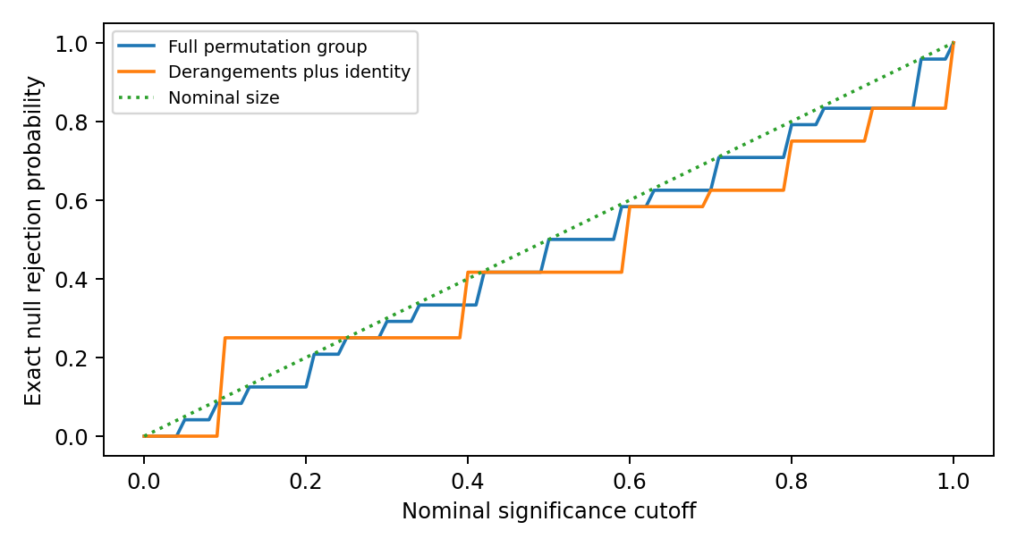
Figure 1. A restricted rearrangement rule can break calibration. The curves enumerate all 24 null pairings, not simulated physical worlds. The dotted line is the nominal upper size bound.
Registration safeguard. Suppose all model optima equal one fixed frame \(D_0\). Matched and mismatched distances are identically zero, so a pairing effect is zero and its p-value is one. This is a recovery control, not an association-positive control. If instead both optima follow a randomly varying supplied orientation, mismatching can give a positive effect without revealing any new dynamical law. Cross-model coordinates need a common operational meaning. Re-expressing each model in its independently supplied frame can remove an apparent effect that only tracked that input.
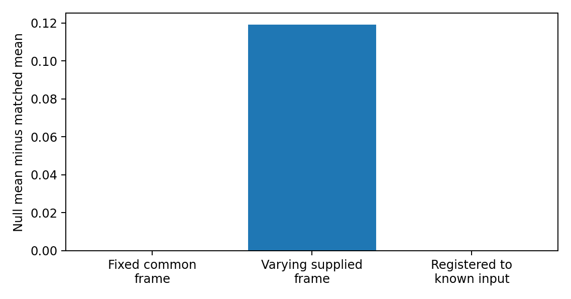
Figure 2. Three exact registration controls. Fixed common frames give zero contrast; differing supplied common orientations give a contrast; registering to those known inputs removes it. This diagnoses the estimand, not an emergent law.
6. Supplied-structure studies and distinct counterfactuals
6.1 Continuously driven calibration
A historical three-qubit study used 20 supplied candidates and a time-averaged singleton-count outcome. Its source coupling and observation window were changed after an initial low-record run, so fresh-seed repeats remain exploratory. Shared preparation, coupling and locality inputs facilitated an apparent overlap enrichment of 0.95 in selected cells. When preparation and coupling moved together, records preferentially remained readable in that supplied frame. These are design-sensitive illustrations, not tests of persistent redundancy or a justified chance-overlap null. Supplement Section S2 preserves the full model, development history, tables and interpretations.
6.2 Source-off pilot: change relative to no evolution
An injection pulse encoded a binary source while internal dynamics were paused. Both source branches then evolved under the same internal Hamiltonian, with the source fully removed. There were 96 independent Hamiltonian/circuit units at each of four and six qubits and two paired injection conditions per unit. The graph, access structures and two comparison frames were supplied. The primary contrast was half the change in the mean singleton trace-distance gap between the native frame L and alternate frame C, averaged over 50 declared positive-time readouts, relative to matched frozen evolution.
The six-qubit rotated-injection mean was -0.015225, with 28 positive and 68 negative units. The approximate bootstrap 95% interval was [-0.021070, -0.009646]; the predeclared range-only interval was [-0.292446, 0.261996]. The observed effect is negative and the bootstrap supports a negative population mean under its sampling approximation, while the conservative range-only bound does not establish its sign at this sample size. The post hoc sign test gives \(p=5.4592\times10^{-5}\) under independent equiprobable nonzero signs; Holm correction across four disclosed conditions gives \(p=1.6377\times10^{-4}\). This is a directional-balance test, not a zero-mean test [Holm 1979]. A negative change narrowed an existing L advantage; it did not make C absolutely superior.
No singleton met the strict new-record criterion throughout an original half-unit window. Some initially uninformative native-frame sites nevertheless became briefly strongly readable. Global distinguishability was conserved and transport controls succeeded. The zero persistent count is conditional on the initial-information floor, singleton access, error threshold and short windows, not absence of information transport.
A separately written review-stage implementation used the declared law with fresh streams, inferring the open-chain convention, circuit-layer order and tensor-factor ordering from the protocol. Those conventions are documented in the accompanying results log. Its 60,000-unit six-qubit rotated sample has mean -0.014125 and a range-only 95% interval [-0.025213, -0.003036]. Re-execution reproduced the supplied output. This strengthens the negative mean for that specific target; it does not identify the mechanism responsible for the change. The reimplementation, historical pilot and subsequent controls are separate runs, not one enlarged original sample.
6.3 Factorial extension: rotating dynamics at fixed injection
The original study held the Hamiltonian native to L. A subsequent exploratory extension supplied the missing alternative intervention, \(H_C=U_C H_L U_C^\dagger\), retaining the same spectrum, unit-specific inputs and readout frames. It crossed injection in \(a\in\{L,C\}\) with evolution under \(b\in\{L,C\}\). For each unit define the post-time-average readability gap \(g_b^a\) and its common initial value \(g_0^a\). Then
\[z_{ab}=\tfrac12(g_b^a-g_0^a),\qquad e_a=z_{aL}-z_{aC}=\tfrac12(g_L^a-g_C^a).\]
The original rotated-pilot target is \(\mathbb E[z_{CL}]\). The new intervention target is \(\mathbb E[e_C]\). The initial gap cancels only in the latter. A negative first quantity and a positive second quantity are fully compatible, not a reversal of one result.
Table 3. Six-qubit factorial extension, 20,000 paired units
| Injection | Dynamics native to L | Dynamics native to C | Paired difference L minus C |
|---|---|---|---|
| L | 0.014004 | 0.003491 | 0.010514 |
| C | -0.014028 | -0.026663 | 0.012635 |
The supplied four-, six- and eight-qubit runs were re-executed. All six mean intervention contrasts are positive. With six disclosed targets and two-sided family coverage at least 95%, the empirical-Bernstein calculation in Supplement Section S4 gives intervals [0.008604, 0.012423] and [0.010692, 0.014579] for the six-qubit L- and C-injection contrasts. Both four-qubit intervals also exclude zero; the eight-qubit intervals with only 1,000 units do not. Normal-approximation intervals are reported separately and are narrower. The analysis is post hoc, assumes independent units from the specified law, and does not certify floating-point error [Maurer and Pontil 2009].
The range is \(e_a\in[-1,1]\), not the loose difference-of-two-ranges interval [-2,2], because the initial gap cancels. This permits the sharper, explicitly derived bound. Its use is a precision calculation for this finite family, not a retrospective preregistration or a guarantee for every analysis selected after review.
6.4 Interpretation and limits
The added factor demonstrates a positive relative effect of the specified Hamiltonian rotation intervention at fixed injection in this family. The old result was a change relative to no evolution; it was not an isolated estimate of a locality mechanism. Neither result is discarded. The independently generated third-frame comparator lies between L and C in the supplied means, but its designation as neutral is a design description, not a theorem that it breaks only one causal link.
Isospectral conjugation does not change only locality: relative to a fixed prepared state it can change energy distributions, correlations with input structure and which observables are simple. Both native and shallow-circuit-rotated Hamiltonians also have controlled finite-range structure relative to related descriptions. Lieb-Robinson bounds constrain commutator propagation under explicit interaction assumptions [Lieb and Robinson 1972]; they do not prove the sign of a difference of time-averaged singleton trace norms. Calling the observed contrast the light-cone effect would therefore be a mechanistic inference requiring further discrimination.
No tensor-product structure is reconstructed by these computations, and the factorial outcome is not strict or redundant record formation. The remaining physical task is to identify unknown structure from several interventions and predict held-out responses without giving the algorithm its target. The methodological lesson is precise: a baseline-subtracted change, a paired Hamiltonian intervention and a structure-identification claim require different evidence.
7. Conjectures and prospective comparisons
Distinct targets. LRA-count compares two declared reference frames, not two independently recovered global optima. It is neither LRA-int nor LRA-tot. The executed source-off pilot instead measures a baseline-subtracted readability change, not persistent record counts. No result is transferred between these targets by renaming it.
7.1 Two distinct model-class hypotheses
An implementation \(\Theta\) must fix a model-history law \(\nu\), source and preparation resources, candidates or search algorithms, record rule, locality rule, valid reference distribution and effect margin. Let \(\mathsf K\) denote that declared population, not a class selected after observing which models make records. For a candidate-overlap design, define \(d_{\Theta,\mathrm{int}}=\mathbb E[A_{\mathrm{int}}-q_{\mathrm{int}}]\) and analogously for the branchwise total score.
LRA-int(\(\Theta\)). \(d_{\Theta,\mathrm{int}}\ge\Delta_{\mathrm{int}}>0\).
LRA-tot(\(\Theta\)). \(d_{\Theta,\mathrm{tot}}\ge\Delta_{\mathrm{tot}}>0\).
Their exact negations are the corresponding strict inequalities below the stated margins. A confidence interval crossing a margin is inconclusive; non-significance is not equivalence. These are conditional model-class hypotheses, not derived theorems of physics. If a frame-distance estimand is chosen instead, it is a different operational hypothesis and receives a separate identifier and margin. One must not switch between the two after seeing results.
The source family \(H_x=H_S+(-1)^xK_{\mathrm C}\) distinguishes internal locality from branchwise total locality. The latter averages separately normalised branch residuals. It is not necessarily the same as a single residual of the joint source-system Hamiltonian: that extension needs its own source-access convention and normalisation. A coupling-dominated example can make LRA-tot descriptively favourable almost by construction. Intermediate \(\kappa=\|H_S\|_{\mathrm{HS}}/\|K_{\mathrm C}\|_{\mathrm{HS}}\) and independent frame variation are therefore useful stress regimes, not guarantees of physical novelty.
7.1.1 Source injection and subsequent redistribution are different questions
For a common initial state \(\rho(0)\) and \(H_x=H_S+K_x\), \[\left.\frac{d}{dt}(\rho_0-\rho_1)\right|_0=-i[K_0-K_1,\rho(0)].\] The common internal generator cancels at first order. This identifies the source of the initial branch difference, not a theorem that one access frame wins at later times. Energy eigenstates selected as pointer states in a regime of weak system-environment interaction in which the system self-Hamiltonian dominates [Paz and Zurek 1999] are also not automatically redundant records of the particular external source bit used here.
A source-off design separates the roles. After a stated injection pulse, set \(K_x=0\) and evolve both branches under the same \(H_S\). Their global trace distance is conserved by that common unitary, while reduced distinguishability can increase, decrease or redistribute. Switching off the source does not remove the prepared imprint. Compare changes against a matched frozen-history control, disclose the supplied injection and readout structures, and distinguish transfer, local accessibility, redundant records and identification of an unknown TPS. The source-off pilot studies this different target, not a relabelling of LRA-count. Its factorial extension additionally varies the Hamiltonian orientation while retaining the specified injection.
Small closed systems can have time-sensitive record windows, but closed dynamics do not preclude persistence: orthogonal stationary product records under a diagonal Hamiltonian remain readable. Conversely, dissipation with one common attractive fixed state can erase the branch distinction. Large size or openness alone is neither a necessary nor a sufficient record guarantee. Environmental many-body interactions can suppress redundancy under the assumptions of Riedel, Zurek and Zwolak (2012). The decoder, retention target and observation window must be specified in each model.
7.2 What an independent search would mean
The locality algorithm may see \(H\) and declared admissibility data, but not record scores. The record algorithm may see conditional states, source and access rules, but not locality scores. Each uses a prospectively fixed optimisation budget and independent random starts. Informational separation of algorithms does not remove shared physical inputs, nor does it prove that either output is a global optimum.
Use multi-start sets rather than pretend there is one unique best frame. Apply an absolute record floor to the original persistent-record target even when a smooth surrogate drives optimisation. A failed search is SEARCH_UNRESOLVED, while a verified absence of qualifying records is NO_RECORD. They have different interpretations and neither supplies a fabricated optimal record frame. Training on some times or histories requires held-out evaluation, and any state-adaptive search lies outside Proposition 3’s fixed-frame union bound.
7.3 Primary prospective target: within-model record contrast
The prospective LRA-count design compares declared frames within each model rather than re-pairing frames across models. It is retained as an unexecuted target, not the primary outcome of the source-off pilot. This is a change of estimand, not a confirmation or falsification of LRA-int or LRA-tot. Let \(E\) denote an input-only eligibility condition, such as separation of the reference frames by a stated \(\Phi\) threshold. For eligible units use \[Z_i=\frac{R_{\mathrm{new}}(D_{L,\mathrm{ref}}(i))-R_{\mathrm{new}}(D_{C,\mathrm{ref}}(i))}{m_{\max}},\qquad \theta_{LC}=\mathbb E[Z_i\mid E=1].\] The common predeclared cap \(m_{\max}\) bounds the admissible disjoint-fragment count. In a singleton study it equals the system-site count. It must not be changed after seeing the records. A reference frame is supplied by the model construction or computed from inputs without record scores. It is not called a unique global optimum unless that is established. In particular the native internal-locality frame need not minimize the total Hamiltonian score. Nonunique references require a predeclared selector, a near-optimal-set sensitivity analysis, or an explicitly supplied-frame interpretation.
The count difference asks how much qualified information distribution differs; the sign contrast \(\mathbb E[\operatorname{sgn}(R_L-R_C)\mid E=1]\) asks how often one frame wins. Both are legitimate but different questions. This unexecuted proposal selects normalized count difference and retains win/loss/tie frequencies as secondary diagnostics. Neither is a causal effect merely because it is called frame attribution.
No-record units remain in the primary denominator with \(Z_i=0\) when absence is established. Define a companion formation indicator using existence of newly qualifying records in the declared union of reference-frame fragment sets. Report its rate on both the complete generated population and the input-eligible population. A formation-conditional contrast is explicitly secondary. When that formation event \(B\) contains every unit with \(Z_i\ne0\), \[\mathbb E[Z\mid E=1]=\Pr(B\mid E=1)\,\mathbb E[Z\mid E=1,B=1].\] Dropping zero-record units therefore changes the magnitude and scientific target. Reference frames remain evaluable even when no record optimum exists. Search failure and unresolved numerical certification are not assigned zero.
Each within-unit comparison is invariant under a consistent common conjugation of its history and access descriptions. This removes cross-model registration and permutation assumptions, but not the need for independent sampling, justified model relevance, resource accounting, fixed thresholds, or honest treatment of uncertainty. A model prepared and coupled in its own reference frame can still favour that frame by design. Separation thresholds and failure of a sufficient perturbation certificate do not prove that a cell is informative.
For a frozen implementation, LRA-count(\(\Theta\)) is \(\theta_{LC}\ge\Delta>0\), with negation \(\theta_{LC}<\Delta\). The sampled class, eligibility law, primary cell, cap, margin and formation diagnostic must be specified before the held-out run. A fully specified negative result counts against this model-class contrast, not every relational ontology. Cross-model pairing remains only a conditional alternative with the explicit contract in the supplement; its counterexamples in Section 5.6 remain valid.
7.3.1 Certification uncertainty must not become a frame advantage
A local reference may have a smaller continuity constant than a scrambled reference. On the same coarse grid, more fragments can then be certified in the local frame even if their true persistent-record counts coincide. That is a property of the certification procedure, not necessarily of the physics. For example, true constant error \(0.099\) is below a \(0.1\) threshold in both frames. A spacing \(0.01\) and valid constants \(0.1\) and \(1\) give upper certificates \(0.0995\) and \(0.104\). The second is unresolved, not a demonstrated absence of a record.
Maintain lower and upper count bounds \(R^{\mathrm{lo}}\le R_{\mathrm{new}}\le R^{\mathrm{hi}}\). Certified fragments provide a lower bound. Every fragment not proved to fail remains eligible for the upper bound; disjoint packing is solved consistently for each bound. Then \[Z_i^{\mathrm{lo}}=(R_L^{\mathrm{lo}} -R_C^{\mathrm{hi}})/m_{\max},\qquad Z_i^{\mathrm{hi}}=(R_L^{\mathrm{hi}}-R_C^{\mathrm{lo}})/m_{\max}.\] For \(N\) independent eligible model-history units, deterministic valid enclosures and an endpoint-inclusive fixed analysis, \[\left[\overline{Z^{\mathrm{lo}}}-h,\overline{Z^{\mathrm{hi}}}+h\right]\cap[-1,1],\qquad h=\sqrt{2\log(2/\alpha)/N},\] covers \(\theta_{LC}\) with probability at least \(1-\alpha\). This follows from Hoeffding applied to the unobserved true \(Z_i\in[-1,1]\) and the inequalities between sample means. No independence of the fragment-level certificates is required. If numerical bounds have a failure probability, add that failure budget explicitly. With no valid classification, use the full possible interval, not deletion of the unit. Larger samples reduce sampling error but cannot remove persistent identification width. A bootstrap alone does not fix that width.
7.4 Controls and staged progression
| Control or stage | Correct expected interpretation | Status in this release |
|---|---|---|
| Fixed common frame | Recover the frame, but pairing contrast is zero | Exact counterexample/calibration executed |
| Varying supplied common orientation | Raw pairing contrast can be positive; disclose and condition on the supplied orientation | Exact projector-span calibration executed |
| Known-input registration | Input-only association can disappear | Exact calibration executed |
| Complete permutation group | Conditional size control under its stated null | Exact four-label enumeration executed |
| Derangements-only reference | Not automatically calibrated | Exact anti-conservative counterexample executed |
| Independent conditional Haar preparation | Small fixed fragments rarely qualify in the stated regime | Source simulations reproduced; bounds retained |
| Persistent versus sampled records | Require a continuum certificate or an explicitly discrete target | Certificate and decoder controls executed, Appendix D |
| Unrestricted independent optimisation | Needs access constraints, convergence study and costed search budget | NOT EXECUTED |
| Physically informative LRA model ensemble | Needs independently motivated model class and valid inference | NOT EXECUTED |
The supplied source-off protocol records the executed feasibility pilot. Unrestricted structure search and a prospectively registered, held-out identification study remain unexecuted. The supplied factorial extension is an executed exploratory intervention study, not that identification stage. No larger study is activated by the existence of this protocol: it first needs an informative target, a justified sampling law and an acceptable certification budget. Any subsequent search requires a separate sensitivity and unresolved-rate assessment.
7.5 Physical correspondence remains a separate claim
An effective graph or a few-body Hamiltonian is not a derived spacetime metric. Existing reconstruction work makes additional assumptions explicit [Cao, Carroll and Michalakis 2017]. A fundamental extension needs a primitive-input ledger and an independent target: geometry, causal propagation, dimensionality, or observation distributions evaluated on data not used to choose the frame. Even successful LRA evidence would support its specified models. It would not automatically establish monism, spatial infinity, plenitude or a conscious ground.
8. Relation to prior work
Subsystems from operational or dynamical criteria.
- Virtual subsystems and generalised TPS. Zanardi’s virtual subsystems and their extension define subsystems through operationally accessible observable algebras [Zanardi 2001; Zanardi, Lidar and Lloyd 2004].
- Minimal scrambling. Zanardi, Dallas, Andreadakis and Lloyd define generalised TPS as dual pairs of an operator subalgebra and its commutant, and select them by minimal short-time information scrambling. The long-time extension uses the long-time average of the algebraic out-of-time-order correlator [Zanardi et al. 2024; Andreadakis, Dallas and Zanardi 2023]. Either criterion could replace or complement \(L\) as a dynamical score. The same audit questions apply, but its class invariance, admissible structure, search distribution and reference calibration must be re-established; the theorems do not transfer unchanged by renaming the score. Andreadakis and Zanardi also define a distance between a tensor-product structure and its image under a unitary channel [Andreadakis and Zanardi 2025]; Section 2.7 distinguishes our span diagnostic from a full access-structure comparison.
- Locality from the spectrum. Cotler, Penington and Ranard study when a Hamiltonian’s spectrum determines a local TPS [Cotler, Penington and Ranard 2019]. Stoica argues that preferred structures built only from the Hamiltonian and state are either not unique or not compatible with observation [Stoica 2022]. Soulas, Franzmann and Di Biagio re-examine both results and argue that the first has been widely misread and the second holds only in a weaker version [Soulas, Franzmann and Di Biagio 2025], a reading Stoica disputes [Stoica 2026]. Loizeau and Sels show that the number of subsystems can be inferred from finite-size corrections to the Gaussian density of states in local models [Loizeau and Sels 2025].
- Scope of this paper. Nothing here depends on how that dispute is resolved. Our candidate structures are declared, and our claims are conditional on the declared reference structure.
Records, objectivity and classicality.
- Decoherence and quantum Darwinism. Decoherence and einselection identify states robust under a given interaction, and quantum Darwinism studies the redundant proliferation of information about them [Zurek 2003; Ollivier, Poulin and Zurek 2004; Zurek 2009].
- Preparation dependence. Zwolak, Quan and Zurek (2010) analyse information acquisition in mixed or misaligned environments under specified decohering interactions. This is direct prior art for readiness dependence, not a new mechanism discovered here. Kumar (2023), an undergraduate thesis, reports loss of a quantum-Darwinism redundancy plateau when environmental subsystem divisions are scrambled. Its mutual-information criterion differs from the present persistent Helstrom formation rule. Ollivier (2022) studies imperfect records and POVMs without singling out a preferred system-environment dichotomy. His construction still assumes microscopic sites and a natural tensor-product structure (Sections 1 and 2); it is not a derivation of arbitrary subsystem structure from no input factorisation. The present Helstrom-persistence test asks a different operational question.
- Genericity. Brandão, Piani and Horodecki proved that the objectivity of observables is generic in quantum dynamics, while the objectivity of outcomes is model-dependent [Brandão, Piani and Horodecki 2015].
- Stronger objectivity notions. Spectrum broadcast structures formalise stronger objectivity [Horodecki, Korbicz and Horodecki 2015]. Their claimed equivalence with strong quantum Darwinism was later qualified in a reply to a published comment [Le and Olaya-Castro 2019, 2021].
- Riedel. Given the TPS of spatial locality, redundant local records constrain branch decompositions strongly [Riedel 2017]. Our question is the converse direction: whether record structure selects that TPS.
- Adil et al. A fixed Hamiltonian admits many factorizations with robust pointer states, and these need not align with the usual notion of locality [Adil et al. 2026]. Their pointer-state criterion is not identical to persistent, redundantly decodable source records. Supplement Table S6 is a separate small illustration of frame sensitivity, not a replication of their stronger or differently defined claims.
Typicality. Proposition 3 is a direct consequence of subsystem-typicality estimates [Page 1993; Popescu, Short and Winter 2006; Goldstein et al. 2006; Hayden, Leung and Winter 2006]. We claim no new typicality result. The contribution is its scoped use as a design constraint on record tests. Conditional Haar typicality suppresses selected small-fragment outcomes; it neither identifies the true preparation of the universe nor forbids adaptive encoding.
Contribution and priority. Section 1.3 states the single contribution list. The underlying projection, commutant, concentration and perturbation tools are standard. Their role here is to prevent three specific mistakes: equating span and access, transferring a verdict between counterfactuals, and treating an unresolved certificate as absent information. The factorial illustration is an outcome of a supplied finite model, not a new theorem that locality always determines record structure. External assessment of novelty and usefulness remains necessary.
9. Limitations, falsifiers and competing interpretations
Limitations.
- Finite dimension, qubit factors, pure conditional states in Proposition 3, a binary source, autonomous Hamiltonians and declared reference structures.
- Proposition 3(v) does not cover candidates chosen after inspecting the state.
- The historical continuously driven toy has three qubits and development-stage tuning. The original source-off pilot has four and six qubits; the later review extensions include eight. All use closed dynamics, supplied frames and restricted observation windows. Mean readability is not redundant-record formation.
- The prospective unrestricted search design is not executed. Several exact statistical, access and persistence components are checked, but component success is not an ensemble result.
- The locality residual measures operator weight relative to a declared span; it is not by itself a propagation velocity or a recovered spacetime geometry.
What would change the claims.
- An error in any proof withdraws the corresponding statement. Numerical agreement supports implementation checks but cannot repair a false general proof.
- For the prospective LRA-count target, an uncertainty-valid interval wholly below its predeclared margin counts against that contrast in its declared eligible population. A structurally built-in positive result does not provide the claimed discrimination. The older LRA-int and LRA-tot overlap hypotheses require their own justified reference null and cannot inherit the count-contrast verdict. Held-out model families and larger systems test generalisation, not the correctness of an already exhibited counterexample.
- Different post hoc interventions do not change the original predeclared estimand. More units sharpen sampling precision but do not identify an otherwise unspecified physical mechanism.
Competing interpretations.
- Einselection. Any positive LRA-tot result may be the familiar statement that pointer observables are selected by the interaction Hamiltonian [Zurek 2003]. An LRA-tot result has further content only where the locality frame of the total Hamiltonian is not the frame of any single designed term.
- Algebraic criteria. Criteria that do not privilege locality, such as minimal scrambling, may select the same frames for different reasons. They should be run as comparators.
10. Data, code and reproducibility
The accompanying Supplementary Information provides the complete run catalogue, parameters, random-stream rules, software environment, pre-execution records and commands. The circulation package contains immutable pilot inputs, per-unit outcomes, raw trajectories, numerical-control scripts and the secondary analyses reported here. Historical exploratory outputs retain their original definitions. Same-code replay and separate numerical implementations are distinguished from external replication; floating-point agreement is not a rigorous interval enclosure. No public persistent deposit or external scientific replication is claimed. All four size/arm pilot summaries, including adverse outcomes, are reported in the accompanying results log.
11. Declarations
The author is responsible for the claims and their final approval. Claude, ChatGPT and a Genspark-mediated review assisted analysis, source retrieval, code, drafting and editing; none is an author, and this assistance is not external peer review. No human-participant data were collected. Funding, competing interests and the final author/correspondence metadata remain subject to author confirmation before submission. The philosophical common-ground inquiry is a separate work; no quantum-information result here is evidence that a conscious or infinite substrate exists.
References
- Adil, A., Rudolph, M. S., Arrasmith, A., Holmes, Z., Albrecht, A., and Sornborger, A. (2026). Search for classical subsystems in quantum worlds. Physical Review D 113, 103535 (2026). https://doi.org/10.1103/vj4x-96fk. Preprint arXiv:2403.10895.
- Andreadakis, F., and Zanardi, P. (2025). Tensor product structure geometry under unitary channels. Quantum 9, 1668. https://doi.org/10.22331/q-2025-03-25-1668
- Andreadakis, F., Dallas, E., and Zanardi, P. (2023). Long-time quantum information scrambling and emergent mereology. arXiv:2312.13386.
- Brandão, F. G. S. L., Piani, M., and Horodecki, P. (2015). Generic emergence of classical features in quantum Darwinism. Nature Communications 6, 7908. https://doi.org/10.1038/ncomms8908
- Cao, C., Carroll, S. M., and Michalakis, S. (2017). Space from Hilbert space: Recovering geometry from bulk entanglement. Physical Review D 95, 024031. https://doi.org/10.1103/PhysRevD.95.024031
- Carroll, S. M., and Singh, A. (2021). Quantum mereology: Factorizing Hilbert space into subsystems with quasiclassical dynamics. Physical Review A 103, 022213. https://doi.org/10.1103/PhysRevA.103.022213
- Cotler, J. S., Penington, G. R., and Ranard, D. H. (2019). Locality from the spectrum. Communications in Mathematical Physics 368, 1267-1296. https://doi.org/10.1007/s00220-019-03376-w
- Goldstein, S., Lebowitz, J. L., Tumulka, R., and Zanghì, N. (2006). Canonical typicality. Physical Review Letters 96, 050403.
- Hayden, P., Leung, D. W., and Winter, A. (2006). Aspects of generic entanglement. Communications in Mathematical Physics 265, 95-117.
- Helstrom, C. W. (1969). Quantum detection and estimation theory. Journal of Statistical Physics 1, 231-252. https://doi.org/10.1007/BF01007479
- Hemerik, J., and Goeman, J. (2018). Exact testing with random permutations. TEST 27, 811-825. https://doi.org/10.1007/s11749-017-0571-1 ; author manuscript https://arxiv.org/abs/1411.7565
- Hoeffding, W. (1963). Probability inequalities for sums of bounded random variables. Journal of the American Statistical Association 58(301), 13-30. https://doi.org/10.1080/01621459.1963.10500830
- Holm, S. (1979). A simple sequentially rejective multiple test procedure. Scandinavian Journal of Statistics 6(2), 65-70. https://www.jstor.org/stable/4615733
- Horodecki, R., Korbicz, J. K., and Horodecki, P. (2015). Quantum origins of objectivity. Physical Review A 91, 032122.
- Kumar, M. (2023). Quantum Darwinism and Preferred Choice of Subsystems. Pitzer Senior Theses, 187. https://scholarship.claremont.edu/pitzer_theses/187/
- Le, T. P., and Olaya-Castro, A. (2019). Strong quantum Darwinism and strong independence are equivalent to spectrum broadcast structure. Physical Review Letters 122, 010403. https://doi.org/10.1103/PhysRevLett.122.010403
- Le, T. P., and Olaya-Castro, A. (2021). Reply to Comment on “Strong quantum Darwinism and strong independence are equivalent to spectrum broadcast structure”. arXiv:2101.10756.
- Lieb, E. H., and Robinson, D. W. (1972). The finite group velocity of quantum spin systems. Communications in Mathematical Physics 28, 251-257. https://doi.org/10.1007/BF01645779
- Loizeau, N., and Sels, D. (2025). Quantum mereology and subsystems from the spectrum. Foundations of Physics 55, 3. https://doi.org/10.1007/s10701-024-00813-2
- Maurer, A., and Pontil, M. (2009). Empirical Bernstein Bounds and Sample Variance Penalization. Proceedings of COLT 2009. arXiv:0907.3740. https://arxiv.org/abs/0907.3740
- Ollivier, H. (2022). Emergence of Objectivity for Quantum Many-Body Systems. Entropy 24(2), 277. https://doi.org/10.3390/e24020277 ; https://arxiv.org/html/2202.06832v1
- Ollivier, H., Poulin, D., and Zurek, W. H. (2004). Objective properties from subjective quantum states: Environment as a witness. Physical Review Letters 93, 220401.
- Page, D. N. (1993). Average entropy of a subsystem. Physical Review Letters 71, 1291. arXiv:gr-qc/9305007
- Paz, J. P., and Zurek, W. H. (1999). Quantum limit of decoherence: Environment induced superselection of energy eigenstates. Physical Review Letters 82, 5181-5185. https://doi.org/10.1103/PhysRevLett.82.5181
- Phipson, B., and Smyth, G. K. (2010). Permutation p-values should never be zero: Calculating exact p-values when permutations are randomly drawn. Statistical Applications in Genetics and Molecular Biology 9(1), Article 39. https://doi.org/10.2202/1544-6115.1585
- Popescu, S., Short, A. J., and Winter, A. (2006). Entanglement and the foundations of statistical mechanics. Nature Physics 2, 754-758. https://doi.org/10.1038/nphys444 The longer author preprint, The foundations of statistical mechanics from entanglement: Individual states vs. averages, arXiv:quant-ph/0511225v3, supplies the explicit concentration Lemma 3 and Eqs. 20 to 22 used in Appendix F. These are related accounts, not independent evidence.
- Riedel, C. J. (2017). Classical branch structure from spatial redundancy in a many-body wave function. Physical Review Letters 118, 120402. arXiv:1608.05377
- Riedel, C. J., Zurek, W. H., and Zwolak, M. (2012). The rise and fall of redundancy in decoherence and quantum Darwinism. New Journal of Physics 14, 083010. https://arxiv.org/abs/1205.3197
- Soulas, A., Franzmann, G., and Di Biagio, A. (2025). On the emergence of preferred structures in quantum theory. arXiv:2512.07468.
- Stoica, O. C. (2022). 3D-space and the preferred basis cannot uniquely emerge from the quantum structure. arXiv:2102.08620. Advances in Theoretical and Mathematical Physics 26(10), 3895-3962. https://doi.org/10.4310/ATMP.2022.v26.n10.a12
- Stoica, O. C. (2026). Comment on “On the emergence of preferred structures in quantum theory” by Soulas, Franzmann, and Di Biagio. arXiv:2603.07674.
- Wilde, M. M. (2019). From classical to quantum Shannon theory. arXiv:1106.1445, version 8.
- Zanardi, P. (2001). Virtual quantum subsystems. Physical Review Letters 87, 077901. https://doi.org/10.1103/PhysRevLett.87.077901
- Zanardi, P., Dallas, E., Andreadakis, F., and Lloyd, S. (2024). Operational quantum mereology and minimal scrambling. Quantum 8, 1406. https://doi.org/10.22331/q-2024-07-11-1406
- Zanardi, P., Lidar, D. A., and Lloyd, S. (2004). Quantum tensor product structures are observable induced. Physical Review Letters 92, 060402. https://doi.org/10.1103/PhysRevLett.92.060402
- Zurek, W. H. (2003). Decoherence, einselection, and the quantum origins of the classical. Reviews of Modern Physics 75, 715-775. https://doi.org/10.1103/RevModPhys.75.715
- Zurek, W. H. (2009). Quantum Darwinism. Nature Physics 5, 181-188. https://doi.org/10.1038/nphys1202
- Zwolak, M., Quan, H. T., and Zurek, W. H. (2010). Quantum Darwinism in non-ideal environments. Physical Review A 81, 062110. https://arxiv.org/abs/0911.4307
Appendix A. Numerical provenance
Supplement Section S1 maps every displayed numerical result to its original script, output key and sample definition. The historical 2,000-draw twirl sample and the separate 1,200-draw calibration target the same exact expectation but are not one enlarged sample. The source-off data, post hoc sign analysis and transport-window diagnostic have distinct run records. Version and file-path details are kept there so that they do not substitute for the scientific argument.
Appendix B. Scope of results
The score, covariance, conditional typicality, continuity and finite-cover statements are mathematical results under their explicit premises. Numerical agreement is corroboration of an implementation, not a proof of the universal statements. The finite-cover result is a concentration-and-net corollary; historical priority is not asserted.
The continuously driven simulations are exploratory and time-averaged. The source-off experiment is a separately specified finite readability pilot. Neither tests the original model-class overlap conjectures or recovers an unknown metric. The proposed persistent count comparison remains a different prospective study. Full-space Haar assumptions are not an empirical preparation model for the universe.
Appendix C. Mixed conditional typicality
Proposition 4. Conditional on design information \(Z=z\) that fixes the candidate frame, let each branch have a unitarily invariant density-operator marginal in dimension \(d=d_Fd_R\). Write \(\mathbb E_z[\cdot]=\mathbb E[\cdot\mid Z=z]\) and \(P_x(z)=\mathbb E_z\operatorname{Tr}\rho_x^2\). Then \[\mathbb E_z\|\rho_{F,x}-I/d_F\|_{\mathrm{HS}}^2=\frac{(d_F^2-1)(dP_x(z)-1)}{d_F(d^2-1)},\] \[b_x(z)=\sqrt{\frac{(d_F^2-1)(dP_x(z)-1)}{d^2-1}},\qquad \mathbb E_z[1/2-p_{\mathrm{err}}]\le\frac{b_0(z)+b_1(z)}4.\] For equal priors and \(\varepsilon<1/2\), \[\Pr(p_{\mathrm{err}}\le\varepsilon\mid Z=z)\le\min\left\{1,\frac{b_0(z)+b_1(z)}{2(1-2\varepsilon)}\right\}.\] Proof. Conditional twirling gives \(\mathbb E_z[\rho_x\otimes\rho_x]=\alpha_z I+\beta_z\mathbb F\), where \(\alpha_z=(d-P_x(z))/[d(d^2-1)]\) and \(\beta_z=(dP_x(z)-1)/[d(d^2-1)]\). Contract with the fragment swap, subtract \(1/d_F\), and use the Schatten-norm comparison and Jensen. The triangle and Markov steps are those of Proposition 3; they do not require branch independence. An unconditional result follows by averaging the conditional bounds. Replacing \(P_x(z)\) by an unconditional purity after selecting a frame need not be valid. \(\square\)
The pure-state case is \(P_x=1\) and reduces to Proposition 3; the maximally mixed case \(P_x=1/d\) gives zero advantage. A four-dimensional calibration with spectrum \((0.55,0.25,0.15,0.05)\) has global purity \(0.39\), exact mean centered fragment Hilbert-Schmidt norm squared \(0.056\), and trace-norm bound \(0.3346640106\). The historical sample of 2,000 random eigenbases gave \(0.0557464152\) for that squared norm, with Monte Carlo standard error \(0.0007264476\). Separately, the 1,200-draw calibration gave \(0.05550839355\), with standard error \(0.00093479233\). Both target the same exact value \(0.056\); the samples and provenance are not interchangeable. This is a check of an explicit finite twirl formula, not a new empirical law or a claim of historical priority.
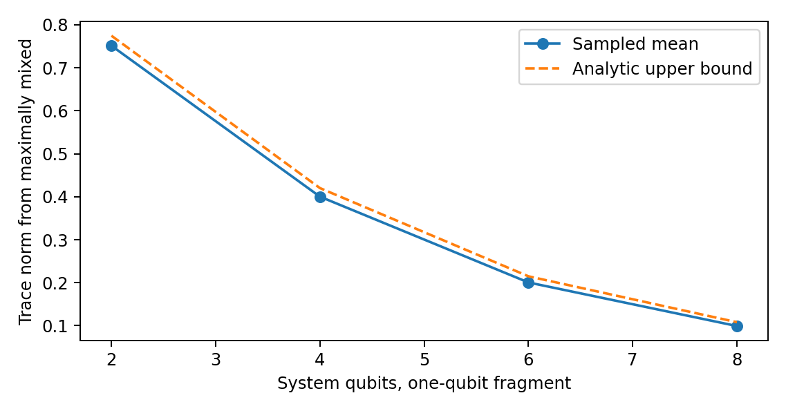
Figure 3. Fixed-fragment typicality calibration. The conditional measure and fragment size are supplied. The bound is not a probability distribution for the universe.
Appendix D. Persistent accessibility and a continuum certificate
Pointwise optimal decoding allows a different measurement at each known time. That is weaker than requiring one fixed decoder when the readout time is unknown. Consider orthogonal Pauli-X eigenstates as source-conditioned states evolving under \(H=Z\). They remain perfectly distinguishable at each known time. At times \(0\) and \(\pi/2\) their labels swap. Averaging over those two unknown times makes both conditional states \(I/2\), so every fixed time-blind decoder has error \(1/2\). A persistence definition must therefore declare whether time, a reference clock and decoder changes are available.
Proposition 5: grid-to-window certificate. For autonomous finite-dimensional conditional generators \(H_x\), define the shift-invariant spectral radius \(\omega_x=\min_{c\in\mathbb R}\|H_x-cI\|_{\mathrm{op}}\). For equal priors and a fixed candidate fragment, \[| p_{\mathrm{err}}^{\mathrm{opt}}(t)-p_{\mathrm{err}}^{\mathrm{opt}}(s)| \le K| t-s| ,\qquad K=(\omega_0+\omega_1)/2.\]
Proof. \(\|\dot\rho_x\|_1=\|[H_x-cI,\rho_x]\|_1\le2\omega_x\). Integrating gives a trace-norm Lipschitz bound, preserved by the partial trace on Hermitian differences. Apply the reverse triangle inequality to the equal-prior Helstrom expression and sum the two branch bounds. The same bound applies to the error of any single fixed binary effect, using that a trace-zero Hermitian difference has maximal effect expectation equal to half its trace norm. \(\square\)
Write \(p_{\mathrm{err}}^{\mathrm{opt}}\) for the pointwise optimal error. On a closed finite window, an endpoint-inclusive grid with largest gap \(h\) and certified grid-error allowance \(\eta_{\mathrm{num}}\) gives \[\max_{t\in T_w}p_{\mathrm{err}}^{\mathrm{opt}}(t)\le\max_j\widehat p_{\mathrm{err}}^{\mathrm{opt}}(t_j)+Kh/2+\eta_{\mathrm{num}}.\] The numerical error budget must be proved or bounded; ordinary floating-point agreement alone is not a rigorous interval enclosure. Where an analytic solution is available it can validate the entire window directly.
For \(H_0=X\), \(H_1=-X\), common initial \(\left| 0\right\rangle\) and \(T_w=[0.70,0.87]\), the analytic error is \((1-\sin2t)/2\). Thirty-five equally spaced points give maximum grid error \(0.0072751350\), \(K=1\) and \(h=0.005\), hence a whole-window upper certificate \(0.0097751350\) before a numerical allowance. The analytic formula also shows one fixed \(Y\) decoder suffices throughout this window. This calibration is distinct from certifying the original three-qubit exploratory table, whose time-averaged outcome is retained as historical data.
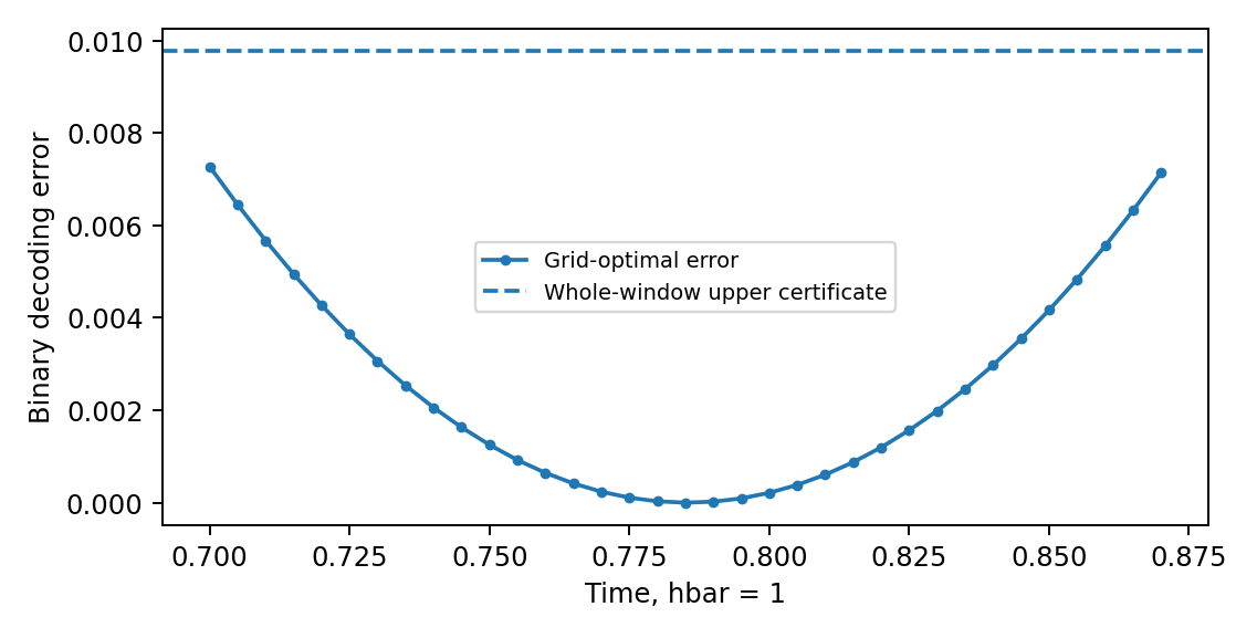
Figure 4. Sampled accessibility is strengthened by an explicit continuity bound. This one-qubit conditional calculation certifies its stated window; it does not certify a different model or an unrestricted frame search.
D.1 Localised certificate without arbitrary term grouping
Proposition 5a. In the coordinates of a fixed candidate, define the normalized conditional expectation onto complement-only operators and the touching part by \[\mathcal E_{\bar F}(H_x)=\frac{I_F}{d_F}\otimes\operatorname{Tr}_F H_x,\qquad H_{x,\mathrm{touch}\, F}=H_x-\mathcal E_{\bar F}(H_x).\] The tensor placement follows the chosen \(F\mid\bar F\) ordering. Put \[\omega_{x,F}=\inf_{c\in\mathbb R}\|H_{x,\mathrm{touch}\, F}-cI\|_{\mathrm{op}},\qquad K_F=(\omega_{0,F}+\omega_{1,F})/2.\] The Lipschitz and grid bounds of Proposition 5 remain valid with \(K_F\). They also remain valid using \(K_{\mathrm{best}}=\tfrac12\sum_x\min(\omega_x,\omega_{x,F})\).
Proof. Complement-only commutators vanish after the partial trace, including on entangled states. Consequently \(\dot\rho_{F,x}=-i\operatorname{Tr}_{\bar F}[H_{x,\mathrm{touch}\, F}-cI,\rho_x]\). The Hermitian operator \(-i[H,\rho]\) obeys trace-norm contraction under partial trace, and \(\|[A,\rho]\|_1\le2\|A\|_{\mathrm{op}}\). Integrate and apply the Helstrom reverse-triangle argument. Both the global and touching bounds hold per branch, so their minima can be used. \(\square\)
An explicit supported-term decomposition gives another valid bound, as follows directly from termwise support. The conditional-expectation form removes arbitrary grouping and cancels all complement-only Pauli components. For fixed-size fragments in bounded-degree models with uniformly bounded incident interactions in the scored frame, the touching bound stays bounded as system size grows. It need not do so for arbitrary nonlocal candidate frames, growing fragments, unbounded couplings or dense graphs. It is not guaranteed smaller than the global bound, hence the minimum above. A tighter derivative bound does not remove decoder or roundoff obligations.
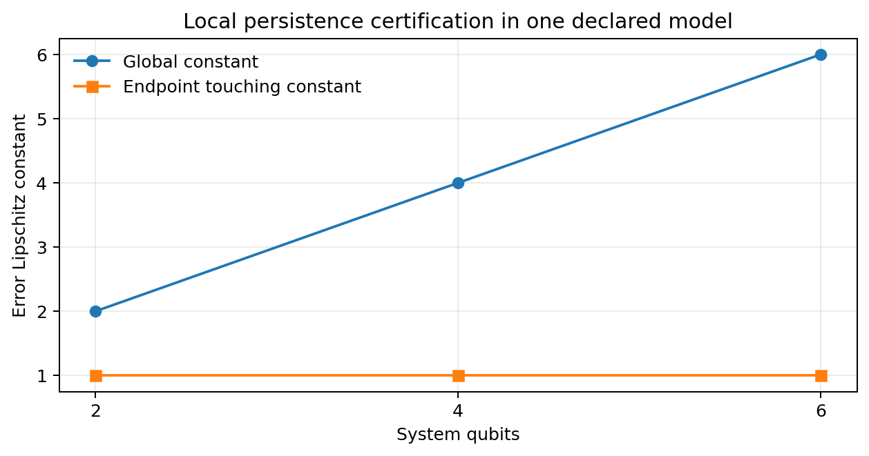
Figure 5. Local certification in a specified model. The new calculation uses \(H_S=0.05\sum_j Z_jZ_{j+1}\) and \(K_x=(-1)^x\sum_j X_j\) for 2, 4 and 6 qubits. The endpoint touching constant is \(\sqrt{1.0025}\) at each size. The conditional expectation removes complement-only terms; the illustration does not prove size independence in every candidate frame.
Appendix E. Perturbation robustness is not a frame-ranking theorem
Proposition 6. For \(H_x=H_S+K_x\) and the same initial conditional states, access and priors, let \(p^0_{\mathrm{err}}(F,t)\) be the optimal error under \(K_x\) alone. In finite dimension, \[|p_{\mathrm{err}}(F,t)-p^0_{\mathrm{err}}(F,t)|\le \left|t\right|\,\omega(H_S),\qquad\omega(H_S)=\inf_c\|H_S-cI\|_{\mathrm{op}}.\] Proof. Subtracting \(cI\) changes only a propagator phase. Duhamel’s formula bounds the operator-norm propagator difference by \(\left|t\right|\|H_S-cI\|\). The corresponding state difference is at most twice that value in trace norm. Reduce to the fragment and apply the weighted Helstrom reverse-triangle inequality. The factor one half cancels the factor two, and the priors sum to one. Minimize over \(c\). \(\square\)
Thus the condition \(p^0_{\mathrm{err}}(F,t)+\left|t\right|\omega(H_S)\le\varepsilon\) at every \(t\in T_w\) is a sufficient preservation certificate for that fragment. It proves neither that this frame minimizes locality nor that it maximizes redundant records, nor that a near-optimal overlap event must occur. Other frames and the full generator’s score still matter. Failure of the sufficient condition does not prove competition: \(H_S=100I\otimes Z\) can have a huge norm while leaving the first qubit’s records under \(K_x=(-1)^xX\otimes I\) unchanged. This exact spectator example is included in the new checks.
Use certified cells as clearly labelled recording controls. Do not remove every norm-dominated cell or call every uncertified cell an informative test by default. A historical 9,000-case numerical check tests the perturbation inequality, not a stronger frame-ranking conclusion; its provenance is retained in the supplement.
Appendix F. Adaptive selection within a predetermined family
Proposition 7 (conditional search-family bound). Condition on design information \(Z=z\). Let both pure branch states have Haar marginals in \(\mathbb C^d\), without requiring joint independence. Fix a nonempty compact unitary family \(\mathcal V_z\) before the realized branch states, and let \(N_z(r)\) be the size of an operator-norm \(r\)-net whose centres lie in that family. Let \(0\le\varepsilon<1/2\), \(r>0\), and \(J\ge1\) declared fragment patterns all have dimension \(d_F\ge2\), with \(d=d_Fd_R\). Put \[b=\sqrt{\frac{d_F^2-1}{d+1}},\qquad a_r=1-2\varepsilon-2r-b>0.\] For equal priors at one specified time, \[\Pr\left(\exists V\in\mathcal V_z,F:\ p_{\mathrm{err}}(F,V)\le\varepsilon\mid Z=z\right)\le\min\left\{1,4J N_z(r)\exp\left[-\frac{d a_r^2}{18\pi^3}\right]\right\}.\] An algorithm may choose its output adaptively from \(\mathcal V_z\); the family itself may not be expanded in response to the realized states without accounting for that expansion. With unequal fragment dimensions use the largest \(b\) or sum the individual bounds.
Proof. For normalized vectors, \(f(\psi)=\|\operatorname{Tr}_{\bar F}\left|\psi\right\rangle\left\langle\psi\right|-I/d_F\|_1\) is at most 2-Lipschitz on the unit sphere. Proposition 3 gives \(\mathbb E_z f\le b\). The explicit version of Levy concentration in Popescu, Short and Winter (2006), Lemma 3 and Eqs. 20 to 22, gives \(\Pr(f\ge b+a)\le2\exp[-d a^2/(18\pi^3)]\) for \(a>0\). This constant uses real sphere dimension \(2d-1\) and the Lipschitz bound two.
For fixed conditional states, \(|p_{\mathrm{err}}(F,V)-p_{\mathrm{err}}(F,W)|\le\|V-W\|_{\mathrm{op}}\): each branch density matrix changes by at most \(2\|V-W\|_{\mathrm{op}}\) in trace norm, and the two branches enter with coefficient one quarter. Therefore a qualifying \(V\) implies a net centre \(W\) with error at most \(\varepsilon+r\). At that centre the triangle bound requires at least one branch deviation \(f_x\ge1-2\varepsilon-2r=b+a_r\). Union over two branches, \(J\) fragments and \(N_z(r)\) centres gives the result. Only marginal Haar concentration is used. \(\square\)
Circuit corollary. For a fixed ordered product of \(P\) gates \(e^{-i\theta_j A_j}\), with fixed Hermitian generators \(\|A_j\|_{\mathrm{op}}\le1\) and \(\theta_j\in[-\Theta,\Theta]\), telescoping bounds unitary distance by \(\sum_j|\theta_j-\theta'_j|\). A coordinate grid of maximum spacing \(2r/P\) gives \[N_z(r)\le(2+2\Theta P/r)^P.\] A finite choice of \(B\) circuit architectures multiplies the cover by at most \(B\). Parameter count alone gives no such bound: parameter ranges, map regularity and allowed architectures matter. This corollary specifies those assumptions rather than using dimension as a substitute for metric entropy.
For \(d=2^n\), fixed fragment dimension and fixed positive \(a_r\), a polynomial log-cover budget is eventually dominated by the \(2^n\) concentration term. The resulting asymptotic suppression has form \(\exp[-\Omega(2^n)]\). This is not a claim of a useful small-\(n\) numerical bound: in the plotted example it remains vacuous over many small system sizes. For the exact Figure 6 settings, the capped bound is one through \(n=18\) and first becomes nontrivial at \(n=19\), with base-ten logarithm approximately \(-56.85\). Even the displayed concentration method without a search cover, for one fixed frame and one singleton with \(r=0\), is capped at one through \(n=10\). Proposition 3 gives the sharper elementary single-fragment bound approximately \(0.525\) at \(n=4\) and \(0.269\) at \(n=6\). These are conditional fixed-frame probabilities, not bounds on all fragments, all times or the non-Haar preparations used in the source-off pilot. Failure to obtain a useful finite-size bound is not a counterexample to the theorem.
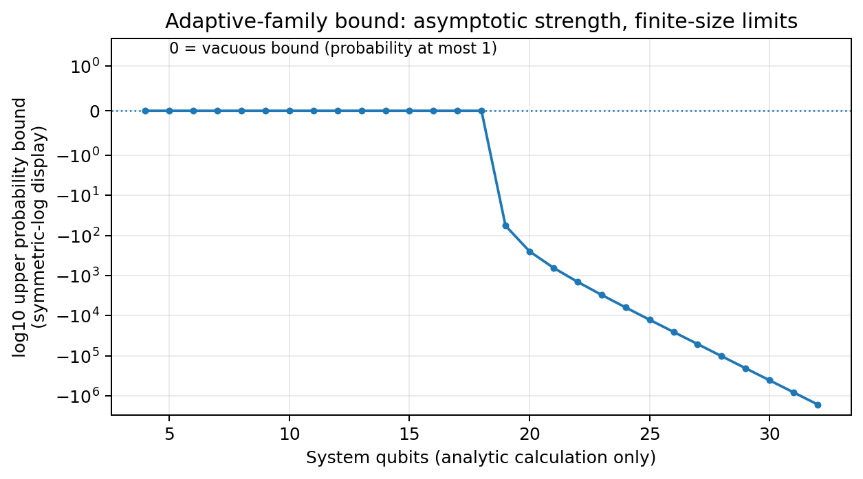
Figure 6. A theorem can be correct while its finite-size bound is uninformative. The plot uses singleton fragments, \(J=n\), \(P=2n\), \(\Theta=\pi\), \(r=0.05\) and \(\varepsilon=0.1\). It displays the base-ten logarithm of the capped bound, with zero meaning probability at most one. The curve is a calculated envelope, not observed record frequencies.
The proposition addresses a uniform-selection question under an explicit covering contract. It is a derived concentration-and-net corollary, not a claim of historical novelty. It does not cover physical energy-shell states, arbitrary nonlinear preparation, a state-chosen family, or every time in a window. Persistent qualification implies qualification at any fixed time in that window, so the same upper bound constrains that event; an existence-at-any-time event needs its own time covering argument. It does not prove emergence of locality or a result about consciousness.